Unveiling Time’s Secrets: A Deep Dive Into Time Series Analysis

P1]

Time series analysis is a powerful statistical technique used to analyze and model data points collected over time. It’s a cornerstone of forecasting, prediction, and understanding the underlying dynamics of various phenomena, ranging from stock prices and weather patterns to website traffic and energy consumption. By understanding the patterns, trends, and dependencies within time-ordered data, we can gain valuable insights and make informed decisions about the future.

This article will explore the core concepts of time series analysis, covering its key components, common techniques, and practical applications. We’ll delve into the intricacies of identifying trends, seasonality, and noise, and discuss how to build predictive models that can accurately forecast future values.

Understanding the Fundamentals:

At its core, time series analysis assumes that past observations influence future values. The data is structured as a sequence of observations, each associated with a specific point in time. This distinguishes it from cross-sectional data, which captures information at a single point in time.

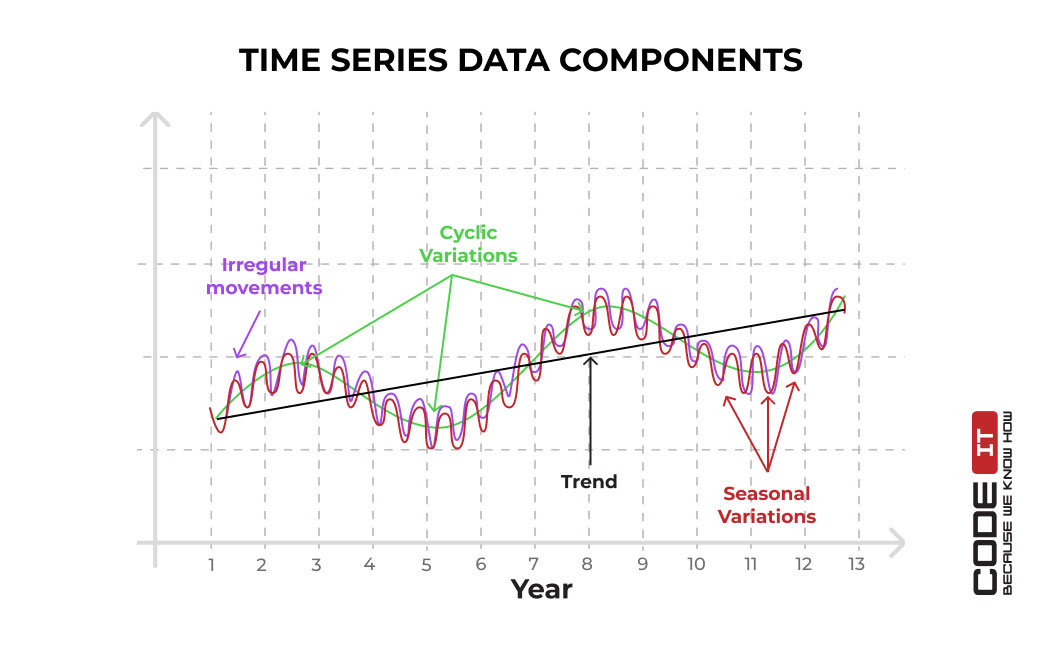
Key components of a time series include:

• Trend: The long-term direction of the data. It can be upward (increasing), downward (decreasing), or stationary (relatively constant). Identifying the trend is crucial for understanding the overall trajectory of the time series.

• 

  Seasonality: Recurring patterns that repeat over fixed intervals, such as daily, weekly, monthly, or yearly cycles. Seasonality is often driven by external factors, like weather conditions, holidays, or business cycles.

• Cyclical Variation: Fluctuations that occur over longer periods than seasonality, typically lasting several years. These cycles are often less predictable than seasonal patterns and can be influenced by economic or political events.



• Irregularity (Noise or Random Variation): Unpredictable fluctuations that don’t follow any discernible pattern. This component represents the inherent randomness in the data and can be challenging to model.

Decomposing Time Series:

One of the first steps in time series analysis is often decomposing the data into its constituent components. This involves separating the trend, seasonality, and residual (irregular) components. Decomposition allows us to isolate each component and analyze it independently.

Several methods exist for decomposition, including:

• Additive Decomposition: Assumes that the components add up to the observed value: Data = Trend + Seasonality + Residual. This is suitable when the magnitude of the seasonal fluctuations is independent of the trend.

• Multiplicative Decomposition: Assumes that the components multiply together to form the observed value: Data = Trend * Seasonality * Residual. This is appropriate when the seasonal fluctuations are proportional to the trend.

• Moving Average Decomposition: Uses moving averages to smooth out the data and estimate the trend. The seasonal component is then calculated by subtracting the trend from the original data.

Essential Techniques for Time Series Analysis:

Once the time series is understood, various techniques can be employed for analysis and forecasting. Some of the most commonly used methods include:

• Moving Averages: Calculates the average of a fixed number of data points to smooth out short-term fluctuations and highlight the underlying trend. Simple Moving Averages (SMA) give equal weight to each data point in the window, while Exponential Moving Averages (EMA) give more weight to recent data.

• Exponential Smoothing: A family of forecasting methods that assigns exponentially decreasing weights to past observations. Different variations of exponential smoothing, such as Simple Exponential Smoothing (SES), Holt’s Linear Trend Method, and Holt-Winters’ Seasonal Method, are suitable for different types of time series data.

• Autoregressive Integrated Moving Average (ARIMA) Models: A powerful class of models that capture the autocorrelations in the data. ARIMA models are defined by three parameters: p (autoregressive order), d (integrated order), and q (moving average order). The p parameter represents the number of lagged values of the time series used as predictors, the d parameter represents the number of times the data needs to be differenced to achieve stationarity, and the q parameter represents the number of lagged forecast errors used as predictors.

• Seasonal ARIMA (SARIMA) Models: An extension of ARIMA models that accounts for seasonality. SARIMA models include additional parameters (P, D, Q, m) to capture the seasonal autoregressive, integrated, and moving average components, where m represents the seasonal period.

• Vector Autoregression (VAR) Models: Used for analyzing multiple time series simultaneously. VAR models capture the interdependencies between different time series and can be used to forecast their future values.

• Prophet: A forecasting procedure developed by Facebook, specifically designed for time series data with strong seasonality and trend. It’s robust to missing data and outliers.

Stationarity: A Critical Concept:

Many time series models, particularly ARIMA models, require the data to be stationary. A stationary time series has constant statistical properties over time, meaning its mean, variance, and autocorrelation structure do not change over time.

Non-stationary time series can be transformed into stationary series using techniques such as:

• Differencing: Subtracting the previous observation from the current observation. This can remove trends and seasonality.

• Log Transformation: Taking the logarithm of the data. This can stabilize the variance.

• Seasonal Adjustment: Removing the seasonal component from the data.

Model Evaluation and Validation:

After building a time series model, it’s crucial to evaluate its performance and validate its accuracy. Common metrics for model evaluation include:

• Mean Absolute Error (MAE): The average absolute difference between the predicted and actual values.

• Mean Squared Error (MSE): The average squared difference between the predicted and actual values.

• Root Mean Squared Error (RMSE): The square root of the MSE.

• Mean Absolute Percentage Error (MAPE): The average absolute percentage difference between the predicted and actual values.

• R-squared: A measure of how well the model fits the data.

Applications of Time Series Analysis:

Time series analysis has a wide range of applications across various domains, including:

• Finance: Predicting stock prices, analyzing market trends, and managing risk.

• Economics: Forecasting economic growth, inflation, and unemployment rates.

• Marketing: Analyzing sales data, forecasting demand, and optimizing marketing campaigns.

• Weather Forecasting: Predicting temperature, rainfall, and other weather conditions.

• Healthcare: Monitoring patient vital signs, predicting disease outbreaks, and optimizing hospital resource allocation.

• Energy: Forecasting energy demand, optimizing energy production, and managing energy grid stability.

• Supply Chain Management: Forecasting demand, optimizing inventory levels, and improving supply chain efficiency.

Challenges and Considerations:

While powerful, time series analysis presents several challenges:

• Data Quality: Accurate and reliable data is essential for building effective models. Missing data, outliers, and measurement errors can significantly impact model performance.

• Model Selection: Choosing the right model for a particular time series can be challenging. Different models have different assumptions and are suitable for different types of data.

• Overfitting: Building a model that fits the training data too well can lead to poor performance on new data. Techniques like cross-validation can help prevent overfitting.

• Interpretability: Some time series models, such as neural networks, can be difficult to interpret. Understanding the underlying mechanisms driving the model’s predictions is crucial for building trust and confidence.

Conclusion:

Time series analysis is a versatile and valuable tool for understanding and predicting temporal data. By mastering the fundamental concepts, techniques, and considerations discussed in this article, you can unlock the power of time series analysis and gain valuable insights from data that evolves over time. From forecasting financial markets to predicting weather patterns, the applications are vast and continue to expand as new data sources and analytical techniques emerge. The key is to understand the specific characteristics of your data and choose the appropriate methods for analysis and prediction.

FAQ – Time Series Analysis

Q1: What is the difference between time series analysis and regression analysis?

• A: While both involve analyzing relationships between variables, time series analysis specifically focuses on data points collected over time. Regression analysis can be applied to various types of data, including cross-sectional data (data collected at a single point in time). Time series analysis also considers the temporal dependencies between observations, which regression analysis typically ignores.

Q2: What does it mean for a time series to be "stationary"?

• A: A stationary time series has constant statistical properties over time. This means its mean, variance, and autocorrelation structure do not change over time. Stationarity is a crucial assumption for many time series models, such as ARIMA models.

Q3: How do I determine if a time series is stationary?

• A: You can visually inspect the time series plot for trends and seasonality. Statistical tests, such as the Augmented Dickey-Fuller (ADF) test and the Kwiatkowski-Phillips-Schmidt-Shin (KPSS) test, can also be used to formally test for stationarity.

Q4: What are some common techniques for making a time series stationary?

• A: Common techniques include differencing (subtracting the previous observation from the current observation), log transformation (taking the logarithm of the data), and seasonal adjustment (removing the seasonal component from the data).

Q5: What is the difference between ARIMA and SARIMA models?

• A: ARIMA models are used for analyzing non-seasonal time series, while SARIMA models are an extension of ARIMA models that account for seasonality. SARIMA models include additional parameters to capture the seasonal autoregressive, integrated, and moving average components.

Q6: How do I choose the appropriate parameters (p, d, q) for an ARIMA model?

• A: The Autocorrelation Function (ACF) and Partial Autocorrelation Function (PACF) plots can help guide the selection of the ARIMA parameters. The ACF plot shows the correlation between a time series and its lagged values, while the PACF plot shows the correlation between a time series and its lagged values after removing the effects of intervening lags. Information criteria, such as AIC and BIC, can also be used to compare different ARIMA models.

Q7: What is cross-validation, and why is it important in time series analysis?

• A: Cross-validation is a technique for evaluating the performance of a model on unseen data. In time series analysis, it involves splitting the data into training and validation sets, training the model on the training set, and evaluating its performance on the validation set. This helps prevent overfitting and provides a more realistic estimate of the model’s performance on future data. Time-series cross-validation requires a specific approach that respects the temporal order of the data (e.g., using rolling or expanding windows).

Q8: What are some common challenges in time series analysis?

• A: Common challenges include data quality issues (missing data, outliers, measurement errors), model selection, overfitting, and interpretability.

Q9: Where can I learn more about time series analysis?

• A: There are many online resources, books, and courses available on time series analysis. Some popular resources include:
  • Online courses on platforms like Coursera, edX, and Udemy.
  • Textbooks on time series analysis and forecasting.
  • Statistical software packages like R, Python, and SAS, which offer extensive libraries for time series analysis.

Q10: What are some real-world examples of time series analysis?

• A: Examples include:
  • Predicting stock prices
  • Forecasting sales
  • Analyzing weather patterns
  • Monitoring patient vital signs
  • Detecting anomalies in network traffic
  • Predicting energy consumption

Conclusion:

Time series analysis provides a robust framework for understanding and forecasting data that evolves over time. Its applications are diverse, ranging from finance and economics to marketing and healthcare. By understanding the fundamental concepts, mastering various techniques, and carefully considering the challenges, practitioners can leverage time series analysis to gain valuable insights, make informed decisions, and ultimately, predict the future with greater accuracy. The continuous development of new algorithms and computing power further enhances the capabilities of time series analysis, making it an increasingly indispensable tool for data-driven decision-making in an ever-changing world. Continuous learning and adaptation to new methodologies are key to staying ahead in this dynamic field.